Kaplan–Meier plots using the ggplot2 package, with an overall Stata-like style. Differences compared to survminer::ggsurvplot() include:
Transparent pointwise confidence interval and simultaneous confidence band areas are always drawn behind survival curves and never over them.
Censor marks are drawn as customizable line segments instead of point symbols.
The risk table title is spaced uniformly with the risk table rows.
The Kaplan–Meier y-axis title remains fixed in place, unaffected by the width of risk table labels.
Installation
You can install the development version of ggKaplanMeier from GitHub with:
remotes::install_github("hongconsulting/ggKaplanMeier")Example: NCCTG lung cancer data
library(ggKaplanMeier)
data <- survival::lung
fig1a <- ggKM(data$time * 12 / 365.2425, data$status - 1, breaks.t = seq(0, 30, 6),
              colors = "#009F6B", title.s = "Overall survival", title.t = "Time (months)")
print(fig1a)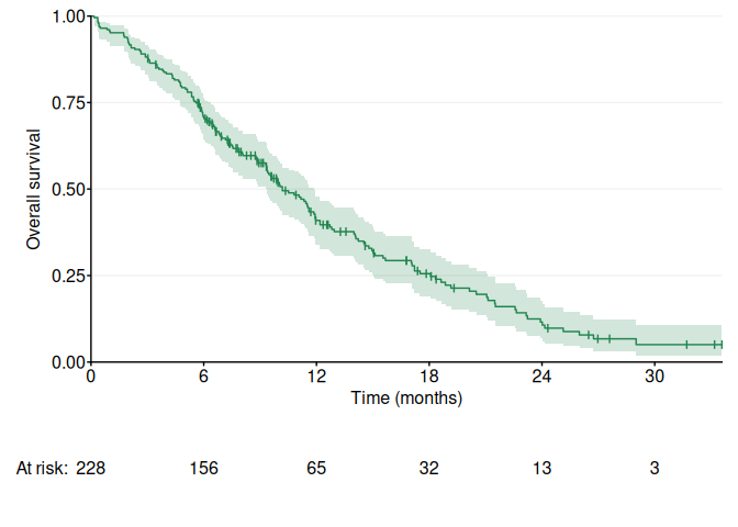
fig1b <- ggKM(data$time * 12 / 365.2425, data$status - 1, data$sex, breaks.t = seq(0, 30, 6), legend.labels = c("Male", "Female"), title.s = "Overall survival", title.t = "Time (months)")
print(fig1b)
print(ggKM.surv.extra(fig1b))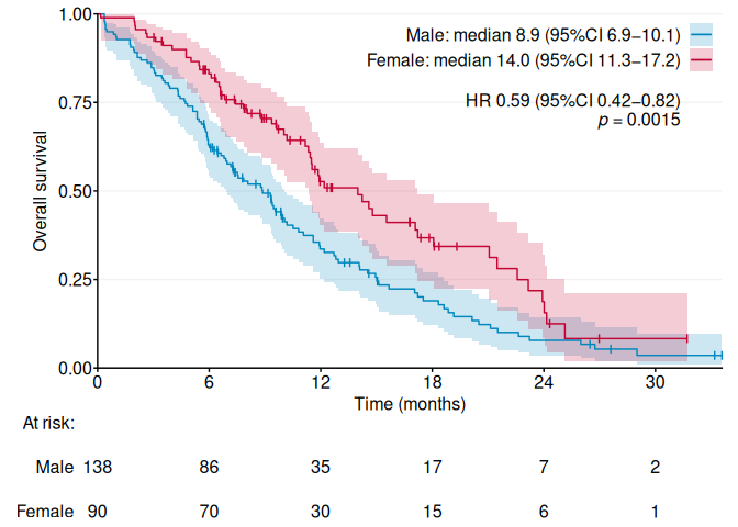
Example: Dukes stage B/C colon cancer study
library(ggKaplanMeier)
data <- survival::colon
fig1 <- ggKM(data$time * 12 / 365.2425, data$status, data$extent,
             colors = c("#0087BD", "#009F6B", "#FEA500", "#C40233"),
             legend.direction = "horizontal", legend.just = "center",
             legend.labels = c("T1", "T2", "T3", "T4"),
             legend.pos = c(0.5, 0.1), risk.table = 2,
             title.s = "Overall survival", title.t = "Time (months)")
print(fig1)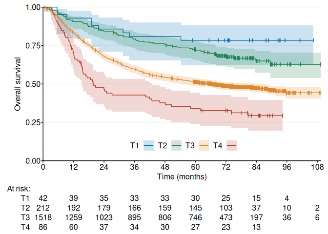
Example: custom CI function
library(ggKaplanMeier)
data <- survival::lung
f.custom <- function() {
  fit <- survival::survfit(survival::Surv(.time, .status) ~ 1,
                           conf.type = "arcsin")
  return(data.frame("time" = fit$time, "surv" = fit$surv,
                    "lower" = fit$lower, "upper" = fit$upper))
}
fig1 <- ggKM(data$time * 12 / 365.2425, data$status - 1, data$sex, CI = f.custom, breaks.t = seq(0, 30, 6), legend.labels = c("Male", "Female"), title.s = "Overall survival", title.t = "Time (months)")
print(fig1)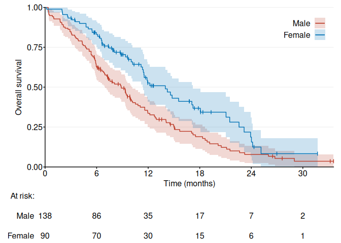
Further Reading
- Brookmeyer, R. and Crowley, J., 1982. A confidence interval for the median survival time. Biometrics, pp. 29–41.
- Cox, D.R., 1972. Regression Models and Life-Tables. Journal of the Royal Statistical Society, Series B. 34(2), pp. 187–220.
- Dorey, F.J. and Korn, E.L., 1987. Effective sample sizes for confidence intervals for survival probabilities. Statistics in Medicine, 6(6), pp. 679–687.
- Fay, M.P., Brittain, E.H. and Proschan, M.A., 2013. Pointwise confidence intervals for a survival distribution with small samples or heavy censoring. Biostatistics, 14(4), pp. 723–736.
- Greenwood, M., 1926. A report on the natural duration of cancer. In: Reports on Public Health and Medical Subjects, 33, pp. 1–26. London: Her Majesty’s Stationery Office, Ministry of Health.
- Hollander, M. and McKeague, I.W., 1997. Likelihood ratio-based confidence bands for survival functions. Journal of the American Statistical Association, 92(437), pp. 215–226.
- Klein, J.P., Logan, B., Harhoff, M. and Andersen, P.K., 2007. Analyzing survival curves at a fixed point in time. Statistics in Medicine, 26(24), pp. 4505–4519.
- Nair, V.N., 1984. Confidence bands for survival functions with censored data: a comparative study. Technometrics, 26, pp. 265–275.
- Rothman, K.J., 1978. Estimation of confidence limits for the cumulative probability of survival in life table analysis. Journal of Chronic Diseases, 31(8), pp. 557–560.
- Thomas, D.R. and Grunkemeier, G.L., 1975. Confidence interval estimation of survival probabilities for censored data. Journal of the American Statistical Association, 70(352), pp. 865–871.