Generates a Kaplan–Meier plot with optional confidence intervals and risk table.
Usage
ggKM(
  time,
  status,
  group = NULL,
  breaks.s = seq(0, 1, 0.25),
  breaks.t = NULL,
  CI = "cloglog",
  CI.alpha = 0.2,
  colors = c("#0087BD", "#C40233", "#009F6B", "#FEA500", "#9755AE", "#33B1BD", "#FFD300",
    "#D8668B"),
  digits.fixed = 1,
  grid.color = grDevices::rgb(0.95, 0.95, 0.95),
  grid.s = seq(0, 1, 0.25),
  grid.t = NULL,
  grid.width = 0.5,
  legend.direction = "vertical",
  legend.just = c("right", "top"),
  legend.label.pos = "left",
  legend.labels = NULL,
  legend.ncol = NULL,
  legend.nrow = NULL,
  legend.pos = c(1, 1),
  legend.text.align = 1,
  margin.KM.b = 0,
  margin.KM.l = 0,
  margin.KM.r = 0,
  margin.KM.t = 4,
  margin.risk = 16,
  line.width = 0.5,
  line.height = 0.025,
  max.t = NULL,
  risk.table = 1,
  risk.table.prop = 0.2,
  t.labels = NULL,
  textsize.axis = 12,
  textsize.legend = 12,
  textsize.risk = 12,
  title.s = "Survival",
  title.t = "Time",
  weights = NULL
)
Arguments
- time
Numeric vector of follow-up times.
- status
Integer vector event indicator (
1= event,0= censored).- group
Optional integer vector grouping variable.
- breaks.s
Y-axis (survival) tick marks. Default =
seq(0, 1, 0.25).- breaks.t
X-axis (time) tick marks. Default =
seq(0, max(time), by = 12).- CI
String indicating the CI type (or a custom function; see Details):
"none": nonePointwise confidence intervals:
"cloglog"(default): Greenwood's variance¹ with complementary log–log transformation²"modcloglog":"cloglog"with the lower confidence limit modified according to the effective sample size at each censored observation³"Rothman": Rothman's binomial method⁴ (via theWHKMconfpackage)"TG": Thomas–Grunkemeier likelihood-ratio method⁵ (via theWHKMconfpackage)"BPCP": beta product confidence procedure⁶ (via thebpcppackage)
Simultaneous confidence bands:
"Nair": Nair's log-transformed equal precision method⁷ (via theWHKMconfpackage)"HM": Hollander–McKeague likelihood-ratio method⁸ (via theWHKMconfpackage)
- CI.alpha
Alpha transparency of the confidence intervals. Default =
0.2.- colors
Vector of colors of the survival curves. Default =
c("#0087BD", "#C40233", "#009F6B", "#FEA500", "#9755AE", "#33B1BD", "#FFD300", "#D8668B").- digits.fixed
Number of decimal places for the risk table if
weightsare used. Default =1.- grid.color
Gridline color. Default =
grDevices::rgb(0.95, 0.95, 0.95).- grid.s
Horizontal gridline positions. Default =
seq(0, 1, 0.25).- grid.t
Vertical gridline positions. Default =
NULL.- grid.width
Gridline thickness. Default =
0.5.- legend.direction
Legend orientation; either
"vertical"(default) or"horizontal".- legend.just
Alignment anchor for the legend relative to its position. Can be a single keyword (e.g.,
"center"), a keyword pair specifying horizontal and vertical justification (e.g.,c("left", "top"),c("right", "bottom")) respectively, or a numeric vector of length 2 giving relative coordinates within the plot area. Default =c("right", "top").- legend.label.pos
Legend label position (
"left"or"right") relative to the legend symbol. Default ="left".- legend.labels
Character vector of group labels.
- legend.ncol
Integer specifying the number of columns in the legend. Default =
NULL.- legend.nrow
Integer specifying the number of rows in the legend. Default =
NULL.- legend.pos
Position of the legend. Can be a keyword such as
"none","left","right","bottom", or"top", or a numeric vector of length 2 giving relative coordinates within the plot area. Default =c(1, 1). Set to"none"ifgroupisNULL.- legend.text.align
Legend text alignment:
0= left,0.5= center,1= right. Default =1.- margin.KM.b
Numeric value specifying the size of the Kaplan–Meier plot bottom margin in points. Default =
0.- margin.KM.l
Numeric value specifying the size of the Kaplan–Meier plot left margin in points. Default =
0.- margin.KM.r
Numeric value specifying the size of the Kaplan–Meier plot right margin in points. Default =
0.- margin.KM.t
Numeric value specifying the size of the Kaplan–Meier plot top margin in points. Default =
4.- margin.risk
Numeric value specifying the horizontal spacing between the risk table labels and the risk table. Default =
16.- line.width
Line width survival curves and censor marks. Default =
0.5.- line.height
Height of censor marks. Default =
0.025.- max.t
Optional numeric value specifying the maximum time up to which the Kaplan–Meier plot and risk table are displayed.
- risk.table
Integer specifying the risk table mode:
0: No risk table1(default): Labelled risk table2: Color-coded risk table
- risk.table.prop
Relative height of the risk table. Default =
0.2.- t.labels
Optional string vector specifying custom labels for the time-axis breaks defined by
breaks.t.- textsize.axis
Axis text size. Default =
12.- textsize.legend
Legend text size. Default =
12.- textsize.risk
Risk table text size. Default =
12.- title.s
Y-axis (survival) title. Default =
"Survival".- title.t
X-axis (time) title. Default =
"Time".- weights
Optional numeric vector of observation weights.
Value
A ggplot (+ patchwork if risk.table ≥ 1) object. The returned
object also stores the processed input time, status, and group as attributes.
A ggplot object (combined with patchwork if risk.table ≥ 1).
The returned object stores additional data as attributes:
Processed input data:
attr(x, "time"): follow-up timesattr(x, "status"): event indicatorattr(x, "group"): grouping variable
Kaplan–Meier estimates (truncated at
max.t):attr(x, "KM_time"): step timesattr(x, "KM_surv"): survival estimatesattr(x, "KM_lower"): lower confidence limitsattr(x, "KM_upper"): upper confidence limitsattr(x, "KM_group"): grouping variable
Details
Observations with invalid time or missing status are automatically
excluded.
A custom function passed to CI is called once per group in an environment
containing the following variables:
.time: Numeric vector of follow-up times for the currentgroup.status: Integer vector event indicator (1= event,0= censored) for the currentgroup.weights: Numeric vector of weights for the currentgroup
The custom function must return a data.frame with the following columns:
$time: times$surv: survival estimate$lower: lower confidence limit$upper: upper confidence limit
References
Greenwood, M., 1926. A report on the natural duration of cancer. In: Reports on Public Health and Medical Subjects, 33, pp. 1–26. London: Her Majesty’s Stationery Office, Ministry of Health.
Klein, J.P., Logan, B., Harhoff, M. and Andersen, P.K., 2007. Analyzing survival curves at a fixed point in time. Statistics in Medicine, 26(24), pp. 4505–4519.
Dorey, F.J. and Korn, E.L., 1987. Effective sample sizes for confidence intervals for survival probabilities. Statistics in Medicine, 6(6), pp. 679–687.
Rothman, K.J., 1978. Estimation of confidence limits for the cumulative probability of survival in life table analysis. Journal of Chronic Diseases, 31(8), pp. 557–560.
Thomas, D.R. and Grunkemeier, G.L., 1975. Confidence interval estimation of survival probabilities for censored data. Journal of the American Statistical Association, 70(352), pp. 865–871.
Fay, M.P., Brittain, E.H. and Proschan, M.A., 2013. Pointwise confidence intervals for a survival distribution with small samples or heavy censoring. Biostatistics, 14(4), pp. 723–736.
Nair, V.N., 1984. Confidence bands for survival functions with censored data: a comparative study. Technometrics, 26, pp. 265–275.
Hollander, M. and McKeague, I.W., 1997. Likelihood ratio-based confidence bands for survival functions. Journal of the American Statistical Association, 92(437), pp. 215–226.
Examples
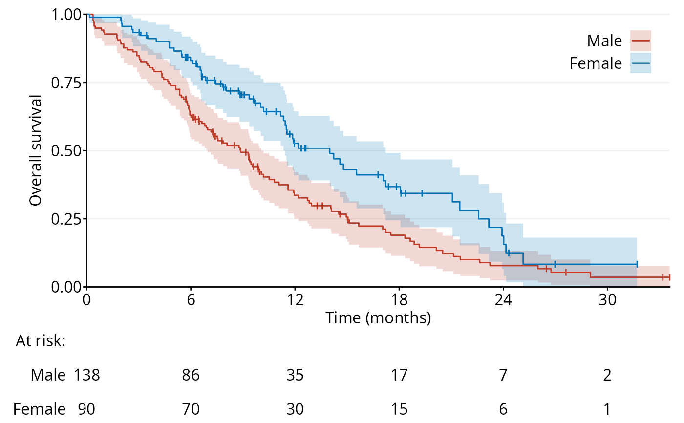
data <- survival::lung
fig1a <- ggKM(data$time * 12 / 365.2425, data$status - 1, data$sex,
breaks.t = seq(0, 30, 6), legend.labels = c("Male", "Female"),
title.s = "Overall survival", title.t = "Time (months)")
print(fig1a)
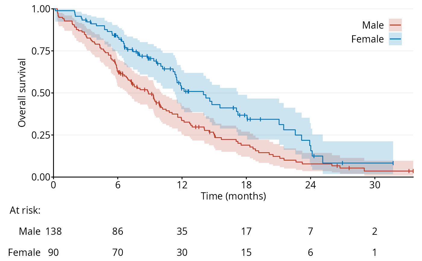 f.custom <- function() {
fit <- survival::survfit(survival::Surv(.time, .status) ~ 1,
conf.type = "arcsin")
return(data.frame("time" = fit$time, "surv" = fit$surv,
"lower" = fit$lower, "upper" = fit$upper))
}
fig1b <- ggKM(data$time * 12 / 365.2425, data$status - 1, data$sex,
breaks.t = seq(0, 30, 6), legend.labels = c("Male", "Female"),
title.s = "Overall survival", title.t = "Time (months)",
CI = f.custom)
print(fig1b)
f.custom <- function() {
fit <- survival::survfit(survival::Surv(.time, .status) ~ 1,
conf.type = "arcsin")
return(data.frame("time" = fit$time, "surv" = fit$surv,
"lower" = fit$lower, "upper" = fit$upper))
}
fig1b <- ggKM(data$time * 12 / 365.2425, data$status - 1, data$sex,
breaks.t = seq(0, 30, 6), legend.labels = c("Male", "Female"),
title.s = "Overall survival", title.t = "Time (months)",
CI = f.custom)
print(fig1b)